Fitting BFACT to Real Climate Data

This vignette demonstrates the complete workflow for fitting the BFACT model to climate data, using New York temperature anomalies as an example.

Introduction

The BFACT package utilizes climate data from:

Climate Models: Temperature anomalies from CMIP6 models for 3 SSP scenarios (1850-2100)
Observations: HadCRUT5 annual temperature anomalies (1850-2022)
Location: This example looks at the New York region, summer (JJA) seasonal averages

Load Real Climate Data

library(BFACT)
library(ncdf4)
library(patchwork)

# Load NetCDF file containing New York temperature anomalies
nc_file <- system.file("data", "NewYork_temperature_anomalies_JJA_all_models_1961-1990baseline.nc", package = "BFACT")
nc_data <- nc_open(nc_file)

# Extract temperature data: dimensions are [lon, lat, year, scenario, model]
temp_data <- ncvar_get(nc_data, "temperature")
years <- ncvar_get(nc_data, "year")
models <- ncvar_get(nc_data, "model")
# Spatially average across lon and lat for each year, scenario, and model
# Result: [year, scenario, model] = [251, 3, 19]
temp_avg <- apply(temp_data, c(3, 4, 5), mean, na.rm = TRUE)

# Extract data for each SSP scenario
# Scenarios: 1=SSP1-2.6, 2=SSP2-4.5, 3=SSP5-8.5
climate_models <- list(
    z126c = temp_avg[, 1, ],
    z245c = temp_avg[, 2, ],
    z585c = temp_avg[, 3, ]
)

# Add model names as column names
for (i in seq_along(climate_models)) {
    colnames(climate_models[[i]]) <- models
}

# Observations are available for years 1-173 (1850-2022)
hadcrut_file <- system.file("data", "hadcrut5_annual.rds", package = "BFACT")
hadcrut5_annual <- readRDS(hadcrut_file)

nc_close(nc_data)

# Data summary
cat("Climate model dimensions:", dim(climate_models$z126c), "\n")

## Climate model dimensions: 251 19

cat("HadCRUT5 observations:", length(hadcrut5_annual), "years\n")

## HadCRUT5 observations: 173 years

Visualize Data

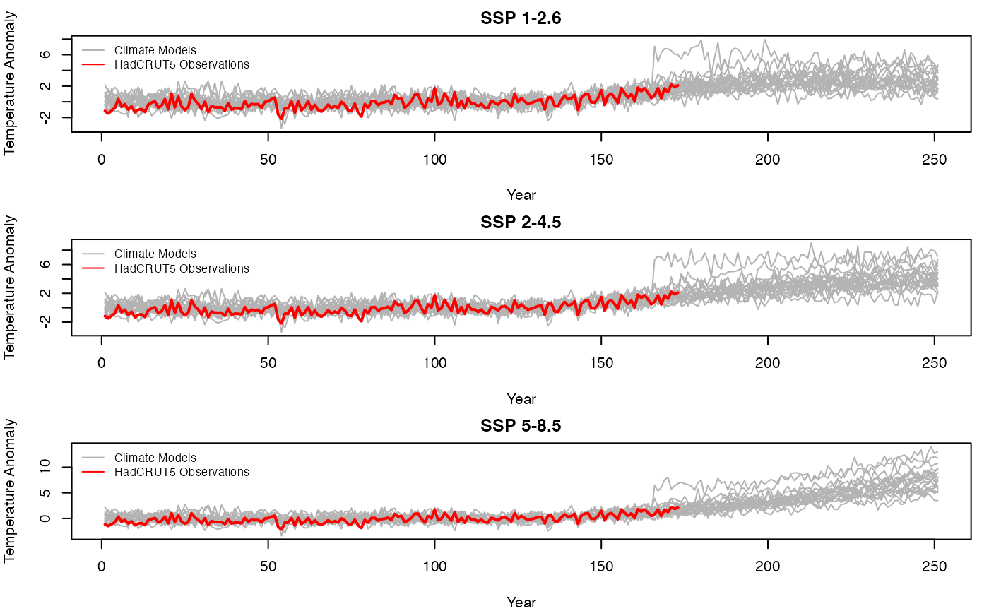
Plot the climate models and observations to see what we’re working with:

par(mfrow = c(3, 1), mar = c(4, 4, 2, 1))
scenarios <- c("z126c", "z245c", "z585c")
titles <- c("SSP 1-2.6", "SSP 2-4.5", "SSP 5-8.5")

for (i in seq_along(scenarios)) {
    mat <- climate_models[[scenarios[i]]]
    matplot(1:nrow(mat), mat,
        type = "l", lty = 1, col = "gray70",
        xlab = "Year", ylab = "Temperature Anomaly", main = titles[i],
        ylim = range(c(mat, hadcrut5_annual), na.rm = TRUE)
    )
    # Add HadCRUT5 observations as red line for overlapping years
    n_hadcrut <- length(hadcrut5_annual)
    lines(1:n_hadcrut, hadcrut5_annual, col = "red", lwd = 2)
    legend("topleft",
        legend = c("Climate Models", "HadCRUT5 Observations"),
        col = c("gray70", "red"), lty = c(1, 1), cex = 0.8, bty = "n"
    )
}

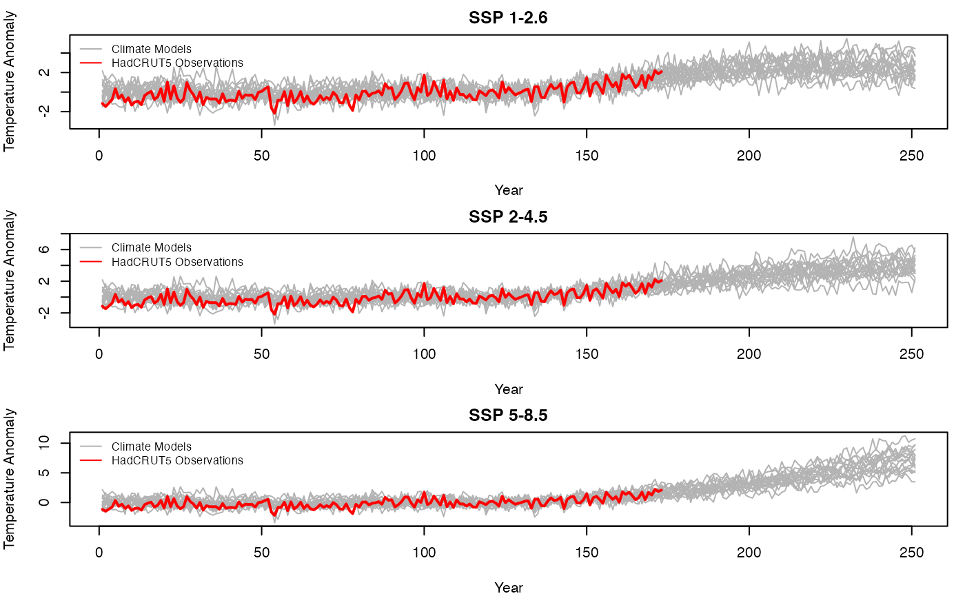
Prune Data for Model Fitting

There are two climate models that are clear outliers in all scenarios. We apply an outlier detection method to identify and remove these models before fitting the BFACT model. This step is performed indpendently for each scenario.

# Apply outlier detection to each scenario and prune
pruned_climate_models <- list()
outlier_models <- list()

for (i in seq_along(scenarios)) {
    mat <- climate_models[[scenarios[i]]]
    outlier_models[[scenarios[i]]] <- BFACT::detect_outliers(
        data = mat,
        start_index = 1,
        end_index = nrow(mat),
        threshold_fn = BFACT::mean_sd_threshold,
        threshold_dial = 2.5
    )
    pruned_climate_models[[scenarios[i]]] <- mat[, !colnames(mat) %in% outlier_models[[scenarios[i]]], drop = FALSE]
}

cat("Outliers by scenario:\n")

## Outliers by scenario:

print(outlier_models)

## $z126c
## [1] "CIESM"       "UKESM1-0-LL"
## 
## $z245c
## [1] "CIESM"       "UKESM1-0-LL"
## 
## $z585c
## [1] "CIESM"       "UKESM1-0-LL"

# Use pruned data for downstream fitting
par(mfrow = c(3, 1), mar = c(4, 4, 2, 1))
climate_models <- pruned_climate_models

for (i in seq_along(scenarios)) {
    mat <- climate_models[[scenarios[i]]]
    matplot(1:nrow(mat), mat,
        type = "l", lty = 1, col = "gray70",
        xlab = "Year", ylab = "Temperature Anomaly", main = titles[i],
        ylim = range(c(mat, hadcrut5_annual), na.rm = TRUE)
    )
    # Add HadCRUT5 observations as red line for overlapping years
    n_hadcrut <- length(hadcrut5_annual)
    lines(1:n_hadcrut, hadcrut5_annual, col = "red", lwd = 2)
    legend("topleft",
        legend = c("Climate Models", "HadCRUT5 Observations"),
        col = c("gray70", "red"), lty = c(1, 1), cex = 0.8, bty = "n"
    )
}

Fit BFACT Models

Fit the BFACT model for each SSP scenario. This demonstration uses 100 MCMC iterations for speed; the full analysis in the paper uses 10000 iterations. Here we fit just H=2 for simplicity.

# Fit BFACT for each SSP scenario
# Note: Using reduced parameters for demonstration
# Paper uses: H=2:7, nsim=10000
results <- list()

for (i in seq_along(scenarios)) {
    cat(sprintf("\n=== Fitting %s ===\n", titles[i]))

    fit <- BFACT(
        Y = climate_models[[scenarios[i]]],
        z = hadcrut5_annual,
        T = 251, # Total time points
        T1 = 1, # Start of climate model data
        T2 = 173, # End of observation data
        H = 2, # Latent factor dimension (paper fits 2:7)
        iseed = 123 + i, # Different seed for each scenario
        J = 6, # Spline basis
        nsim = 100 # MCMC iterations (paper uses 10000)
    )
    results[[scenarios[i]]] <- fit

    cat(sprintf("Completed fit for %s\n", titles[i]))
}

## 
## === Fitting SSP 1-2.6 ===
## Completed fit for SSP 1-2.6
## 
## === Fitting SSP 2-4.5 ===
## Completed fit for SSP 2-4.5
## 
## === Fitting SSP 5-8.5 ===
## Completed fit for SSP 5-8.5

nsim: Number of MCMC iterations (100 here for speed, 10000 in the paper)
J: Spline basis
H: Latent factor dimension (2-7 in full analysis)

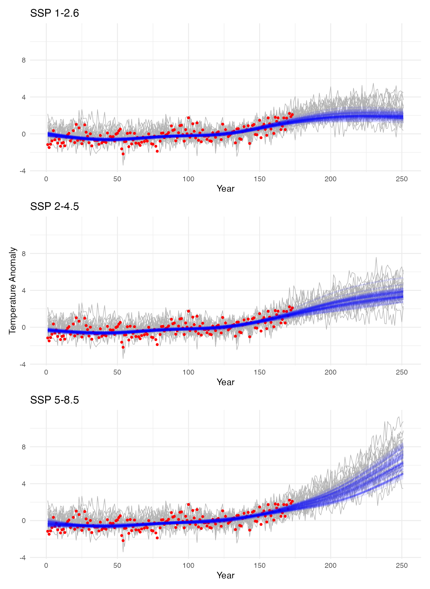
Visualize Posterior Results

Plot the posterior samples against the observations and models:

# Generate plots for each scenario with shared y-axis
plots <- list()

# Calculate shared y-axis limits across all scenarios
all_values <- list()
for (i in seq_along(scenarios)) {
    all_values[[i]] <- c(climate_models[[scenarios[i]]], hadcrut5_annual)
}
shared_ylim <- range(unlist(all_values), na.rm = TRUE)

for (i in seq_along(scenarios)) {
    # Get posterior samples
    fit <- results[[scenarios[i]]]
    burn_start <- ceiling(nrow(fit$beta_samples) / 2)

    # Compute posterior means for each sample
    post_samples <- sample_posterior(fit)

    # Create plot using the new function with shared y-axis limits
    p <- plot_data_with_posterior(
        Y = climate_models[[scenarios[i]]],
        z = hadcrut5_annual,
        posterior_samples = post_samples,
        title = titles[i],
        years = 1:251,
        obs_years = 1:173,
        ylim = shared_ylim
    )

    # Only keep y-axis label on the middle plot
    if (i != 2) {
        p <- p + ggplot2::labs(y = NULL)
    }

    plots[[i]] <- p
}

# Combine plots with patchwork
combined_plot <- plots[[1]] / plots[[2]] / plots[[3]]
print(combined_plot)

Fitting BFACT to Real Climate Data

BFACT Package

2026-02-22