Generate Posterior Simulations

This vignette shows how to generate synthetic climate data from fitted posteriors, then fit BFACT to evaluate model sensitivity.

Workflow:

Extract posterior samples from a model fitted to real data (e.g., $H_0 = 2$ )
Utilize parameters from these posterior samples to generate synthetic climate trajectories
Fit BFACT with multiple $H$ values (1-20) to the synthetic data

Step 1: Fit Real Data and Extract Posterior Samples

Start by fitting BFACT to the real New York temperature data, then extract posterior draws. Here $H_0 = 2$ .

library(BFACT)
library(ncdf4)
library(dplyr)

# Load real climate data (same as vignette 01)
nc_file <- system.file("data", "NewYork_temperature_anomalies_JJA_all_models_1961-1990baseline.nc", package = "BFACT")
nc <- nc_open(nc_file)

temp_data <- ncvar_get(nc, "temperature")
years <- ncvar_get(nc, "year")
models <- ncvar_get(nc, "model")
temp_avg <- apply(temp_data, c(3, 4, 5), mean, na.rm = TRUE)

# Use SSP 5-8.5 (highest warming scenario)
Y_real <- temp_avg[, 3, ]

# Add model names as column names - this is necessary for outlier detection and later analysis
colnames(Y_real) <- models

# Remove outlier models
outliers <- BFACT::detect_outliers(
    data = Y_real,
    start_index = 1,
    end_index = nrow(Y_real),
    threshold_fn = BFACT::mean_sd_threshold,
    threshold_dial = 2.5
)
if (length(outliers) > 0) {
    cat("Removed outlier models:", paste(outliers, collapse = ", "), "\n")
    Y_real <- Y_real[, !colnames(Y_real) %in% outliers, drop = FALSE]
}

## Removed outlier models: CIESM, UKESM1-0-LL

hadcrut_file <- system.file("data", "hadcrut5_annual.rds", package = "BFACT")
z_real <- readRDS(hadcrut_file)

nc_close(nc)

# Fit BFACT to real data with H0=2
cat("Fitting BFACT to real data (H0=2)...\n")

## Fitting BFACT to real data (H0=2)...

fit_real <- BFACT(
    Y = Y_real,
    z = z_real,
    T = 251,
    T1 = 1,
    T2 = 173,
    H = 2,
    iseed = 123,
    J = 6,
    nsim = 100
)

Step 2: Generate Synthetic Data from Posterior Samples

# Generate synthetic data from this posterior draw
sim_posterior <- simulate_from_posterior(
    fit = fit_real,
    years_start = 1850,
    years_end = 2100,
    T1 = 1,
    T2 = 173,
    J = 6,
    OBS_COL = 1,
    seed = 123
)

cat("Real data fit complete. Generated synthetic observations from H0=2 posterior.\n")

## Real data fit complete. Generated synthetic observations from H0=2 posterior.

# Plot simulated data with true trend
p_sim <- plot_data_with_posterior(
    Y = sim_posterior$Y,
    z = sim_posterior$z,
    true_trend = sim_posterior$mu[, 1],
    title = "Synthetic Data: Generated from H0=2 Posterior",
    years = sim_posterior$years,
    obs_years = sim_posterior$T1:sim_posterior$T2
)
p_sim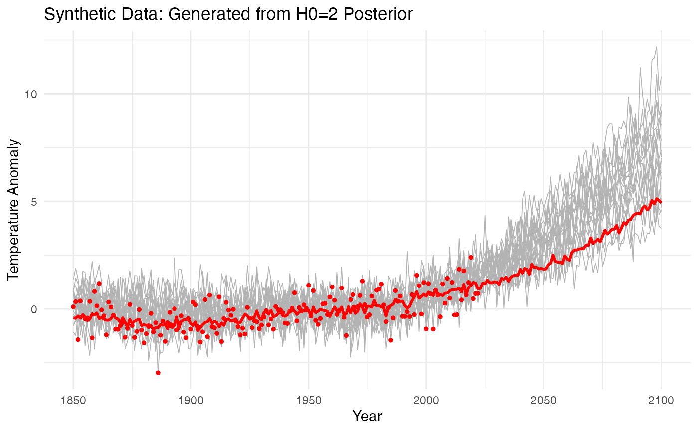

Step 3: Fit Multiple H Values to Synthetic Data

Now fit BFACT with $H \in 2,\ldots,5$ to evaluate model sensitivity:

# Fit H=2 to H=5 to the synthetic data
H_fit_range <- 2:5
fits_posterior <- list()

for (H in H_fit_range) {
    cat(sprintf("\nFitting H=%d to synthetic data from H=2 posterior...\n", H))

    fit <- BFACT(
        Y = sim_posterior$Y,
        z = sim_posterior$z,
        T = 251,
        T1 = 1,
        T2 = 173,
        H = H,
        iseed = 123 + H,
        J = 6,
        nsim = 100
    )

    fits_posterior[[as.character(H)]] <- fit
}

## 
## Fitting H=2 to synthetic data from H=2 posterior...
## 
## Fitting H=3 to synthetic data from H=2 posterior...
## 
## Fitting H=4 to synthetic data from H=2 posterior...
## 
## Fitting H=5 to synthetic data from H=2 posterior...

cat("Completed fits for H=2:5\n")

## Completed fits for H=2:5

Plotting Posterior Fits

library(patchwork)

# Generate posterior fit plots for each H
plots_H <- list()

for (H in H_fit_range) {
    fit <- fits_posterior[[as.character(H)]]

    plots_H[[as.character(H)]] <- plot_data_with_posterior(
        Y = sim_posterior$Y,
        z = sim_posterior$z,
        posterior_samples = sample_posterior(fit),
        title = sprintf("H = %d", H),
        years = sim_posterior$years,
        obs_years = sim_posterior$T1:sim_posterior$T2
    )

    # Only keep y-axis label on the middle plot
    if (H != 3) {
        plots_H[[as.character(H)]] <- plots_H[[as.character(H)]] + ggplot2::labs(y = NULL)
    }
}

# Combine plots in grid
grid_plot <- plots_H[[1]] / plots_H[[2]] / plots_H[[3]] / plots_H[[4]]
print(grid_plot)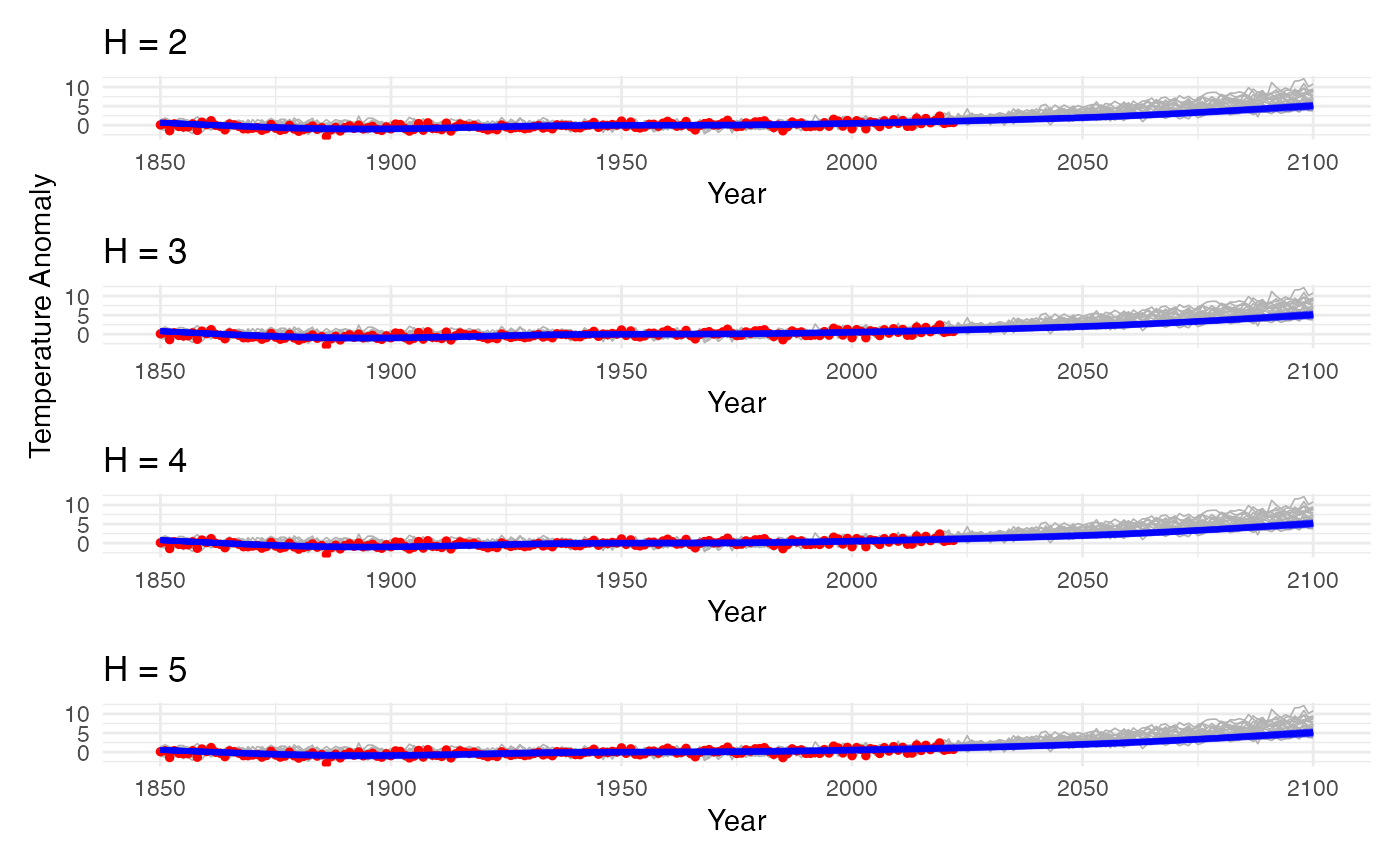

Step 4: Model Sensitivity to H

Compute RMSE for each $H$ value and assess.

out <- consolidate_results(fits_posterior, sim_posterior)

cat("\nModel comparison (RMSE on synthetic data):\n")

## 
## Model comparison (RMSE on synthetic data):

print(out$model_comparison)

## # A tibble: 4 × 4
##       H  RMSE mean_post_var max_post_var
##   <int> <dbl>         <dbl>        <dbl>
## 1     2 0.239       0.0102        0.0530
## 2     3 0.260       0.00960       0.0516
## 3     4 0.258       0.0102        0.0483
## 4     5 0.223       0.0126        0.0520