Model Selection Across Multiple Replications
BFACT Package
2026-02-23
Source:vignettes/03-multiple-replicates.Rmd
03-multiple-replicates.RmdModel Selection Across Multiple Replications
This vignette demonstrates how to assess model selection performance (finding the true H) across multiple independent replications of the data.
We will:
- Generate synthetic data with known true value
- Create 3 independent replications
- Fit BFACT with to each replicate
- Aggregate results across replications using
consolidate_results() - Show summary statistics on model selection
Steps 1 & 2: Generate Multiple Replications
We’ll generate 3 replications of synthetic data from a true model, using different random seeds:
# Generate synthetic data from real posterior
nc_file <- system.file("data", "NewYork_temperature_anomalies_JJA_all_models_1961-1990baseline.nc", package = "BFACT")
nc <- nc_open(nc_file)
temp_data <- ncvar_get(nc, "temperature")
years <- ncvar_get(nc, "year")
models <- ncvar_get(nc, "model")
temp_avg <- apply(temp_data, c(3, 4, 5), mean, na.rm = TRUE)
Y_real <- temp_avg[, 3, ]
colnames(Y_real) <- models
# Remove outlier models
outliers <- BFACT::detect_outliers(
    data = Y_real,
    start_index = 1,
    end_index = nrow(Y_real),
    threshold_fn = BFACT::mean_sd_threshold,
    threshold_dial = 2.5
)
if (length(outliers) > 0) {
    cat("Removed outlier models:", paste(outliers, collapse = ", "), "\n")
    Y_real <- Y_real[, !colnames(Y_real) %in% outliers, drop = FALSE]
}
## Removed outlier models: CIESM, UKESM1-0-LL
climate_models <- list(z585c = Y_real)
hadcrut_file <- system.file("data", "hadcrut5_annual.rds", package = "BFACT")
hadcrut5_annual <- readRDS(hadcrut_file)
nc_close(nc)

# Fit to real data to get a posterior draw
cat("Fitting BFACT to real data to generate posterior...\n")
## Fitting BFACT to real data to generate posterior...
fit_real <- BFACT(
    Y = climate_models$z585c,
    z = hadcrut5_annual,
    T = nrow(climate_models$z585c),
    T1 = 1,
    T2 = length(hadcrut5_annual),
    H = 2,
    iseed = 999,
    J = 6,
    nsim = 100
)

# Generate 3 replications from the posterior
n_reps <- 3
sims_list <- list()
for (rep in 1:n_reps) {
    cat(sprintf("Generating replicate %d/%d...\n", rep, n_reps))
    sim_rep <- simulate_from_posterior(
        fit_real,
        s = NULL, # Random sample from second half of chain
        seed = 1000 + rep
    )
    sims_list[[rep]] <- sim_rep
}
## Generating replicate 1/3...
## Generating replicate 2/3...
## Generating replicate 3/3...## Generated 3 replications with H_true = 2Step 3: Fit BFACT with Multiple H Values to Each Replicate
Now fit H=2, H=3, and H=4 to each replicate:
H_values <- 2:4
fits_list <- list()

for (rep in 1:n_reps) {
    cat(sprintf("\n=== Replicate %d/%d ===\n", rep, n_reps))
    sim_rep <- sims_list[[rep]]
    fits_rep <- list()

    for (H in H_values) {
        cat(sprintf("  Fitting H=%d...\n", H))
        fit <- BFACT(
            Y = sim_rep$Y,
            z = sim_rep$z,
            T = sim_rep$T,
            T1 = sim_rep$T1,
            T2 = sim_rep$T2,
            H = H,
            iseed = 2000 + rep * 100 + H,
            J = 6,
            nsim = 50
        )
        fits_rep[[as.character(H)]] <- fit
    }
    fits_list[[rep]] <- fits_rep
}
##
## === Replicate 1/3 ===
## Fitting H=2...
## Fitting H=3...
## Fitting H=4...
##
## === Replicate 2/3 ===
## Fitting H=2...
## Fitting H=3...
## Fitting H=4...
##
## === Replicate 3/3 ===
## Fitting H=2...
## Fitting H=3...
## Fitting H=4...
cat("\nCompleted all fits!\n")##
## Completed all fits!Step 4: Consolidate Results Across Replications
Use consolidate_results() to aggregate across
replications:
results_multi <- consolidate_results(
    fits = fits_list,
    sim = sims_list,
    by_replicate = TRUE
)
## # A tibble: 3 × 8
## H mean_RMSE sd_RMSE min_RMSE max_RMSE n_reps mean_post_var max_post_var
## <int> <dbl> <dbl> <dbl> <dbl> <int> <dbl> <dbl>
## 1 2 0.292 0.0463 0.241 0.331 3 0.0290 0.0683
## 2 4 0.308 0.0520 0.262 0.364 3 0.0124 0.0157
## 3 3 0.468 0.268 0.289 0.776 3 0.0565 0.148
# View the replicate comparison table
cat("\n=== Model Selection Summary Across Replications ===\n")
##
## === Model Selection Summary Across Replications ===
print(results_multi$replicate_comparison)## # A tibble: 3 × 8
## H mean_RMSE sd_RMSE min_RMSE max_RMSE n_reps mean_post_var max_post_var
## <int> <dbl> <dbl> <dbl> <dbl> <int> <dbl> <dbl>
## 1 2 0.292 0.0463 0.241 0.331 3 0.0290 0.0683
## 2 4 0.308 0.0520 0.262 0.364 3 0.0124 0.0157
## 3 3 0.468 0.268 0.289 0.776 3 0.0565 0.148Step 5: Identify the Elbow Point
Use the elbow method to identify the optimal H value where performance plateaus:
# Extract H values and mean RMSE
H_vals <- results_multi$replicate_comparison$H
rmse_vals <- results_multi$replicate_comparison$mean_RMSE

# Find the elbow
elbow_H <- find_elbow(H_vals, rmse_vals, minimize = TRUE)

cat(sprintf("\nElbow point identified at H = %d\n", elbow_H))
##
## Elbow point identified at H = 2
cat(sprintf(
"Mean RMSE at H=%d: %.4f\n", elbow_H,
results_multi$replicate_comparison$mean_RMSE[
results_multi$replicate_comparison$H == elbow_H
]
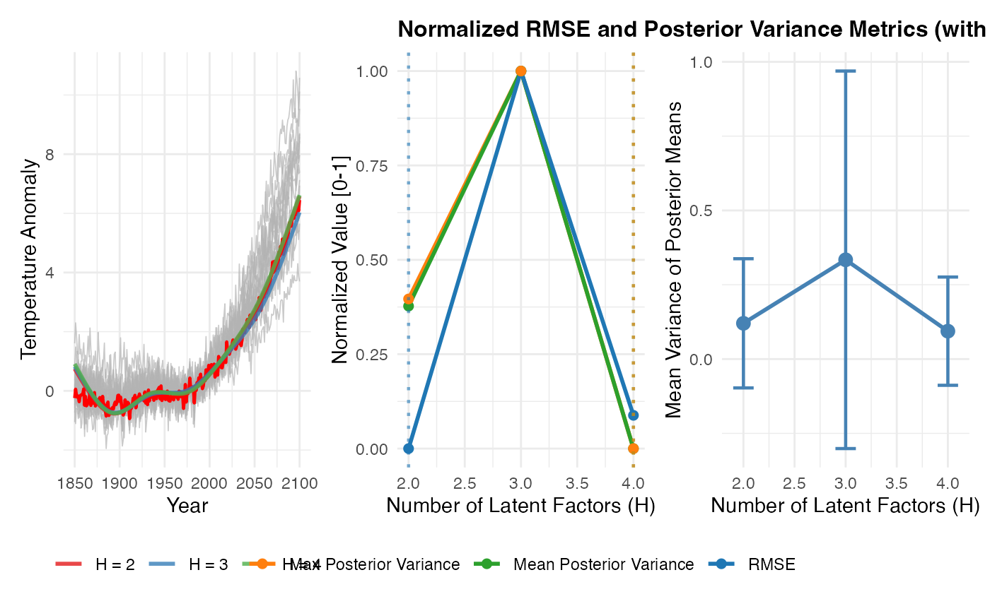
))## Mean RMSE at H=2: 0.2924Step 6: Visualize Model Selection Performance with Elbow
Plot RMSE by H across replications with elbow point marked:
p_avg <- plot_replicate_averages(results_multi, sims_list)
p_norm <- plot_normalized_metrics(
    results_multi$replicate_comparison,
    title = "Normalized RMSE and Posterior Variance Metrics (with Elbow Detection)"
)
p_var <- plot_posterior_variance(results_multi)

combined_plot <- p_avg | p_norm | p_var
print(combined_plot)